This page provides a short overview of the mathematics and models used in the code. We first introduce the basic components of a DPM simulation (global parameters and variables, properties of particles, walls, boundaries, force laws and interactions), and provide the notation used henceforth. Then we explain the basic steps taken in each simulation (setting initial conditions, looping through time, writing data). The document is structured similarly to the code, so the user can easily relate the relevant classes with their purpose. Throughout this text, we include references to the relevant classes and functions, so the user can view the implementation.

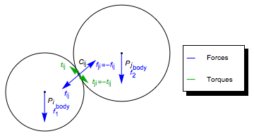
Basic components of a DPM simulation

In its most basic implementation, a DPM simulation simulates the movement of a set of particles $P_i,\ \ i=1,\dots,N$, each of which is subject to body forces $\vec f_i^\mathrm{body}$ and interacts with other particles via interaction forces $\vec f_{ij}$, and torques $\vec t_{ij},\ \ i=1,\dots,N_\mathrm{interaction}$.

While the body forces are assumed to act in the particle's center of mass $\vec r_i$, the interaction forces act at the contact point $\vec c_{ij}$ between the particles. Thus, each particle is subjected to the total force and torque

\[\vec f_i = \vec f_i^\mathrm{body}+\sum_{j=1}^N \vec f_{ij},\quad \vec t_i = \sum_{j=1}^N \vec t_{ij} + (\vec{c}_{ij}-\vec{r}_i)\times \vec f_{ij}.\]

Sketch of two contacting particles, showing body and interaction forces.

To simulate the movement of each particle, the particles' initial properties are defined, then Newton's laws are applied, resulting in the equations of motion,

\[m_i \ddot{\vec{r_i}} = \vec f_i,\quad I_i \dot{\vec{\omega_i}} = \vec t_i,\]

where $m_i$, $I_i$, $\omega_i$ are the mass, moment of inertia and angular velocity of each particle (we currently do not use the particles' orientation, as all particles are spherical).

The default body force applied to a particle is due to gravity, $\vec f_i^\mathrm{body}=m_i \vec{g}$, with $\vec g$ the gravitational acceleration. The interaction forces can be quite varied, but usually consist of a repulsive normal force due to the physical deformation when two particles are in contact, and possibly an adhesive normal force

\[\vec f_{ij} = (f_{ij}^{n,rep}-f_{ij}^{n,rep})\vec n_{ij} + \vec f_{ij}^{t},\]

with $\vec n_{ij}$ the normal direction at the contact point, which for spherical particles is given by $\vec n_{ij}=\frac{\vec r_j-\vec r_i}{|\vec r_j-\vec r_i|}$.

Further, a set of walls $W_j,\ \ j=1,\dots,N$ can be implemented, which can apply an additional force $\vec f_{ij}$ and torque $\vec t_{ij}$ to each particle $P_i$. A typical, flat wall is defined by

\[\mathrm{W}_j = \{\vec{r}:\ \vec{n}_j \cdot (\vec{r} - \vec{r}_j) \leq 0 \},\]

with $ \vec{n}_j$ the unit vector pointing into the wall and $\vec{r}_j$ a point on the wall. However, many other wall types are possible, such as intersections of planar walls (e.g. polyhedral walls), axisymmetric walls (e.g., cylinders or funnels), or even complex shapes (coils and helical walls).

More complex simulations include further boundary conditions $B_j,\ \ j=1,\dots,N$, such as periodic walls and regions where particles get destroyed or added.

Time integration is done using Velocity Verlet, see http://en.wikipedia.org/wiki/Verlet_integration#Velocity_Verlet for details. The implementation can be found in DPMBase::solve.

Variables

In the following sections, we give a short overview over the parameters that can be specified in MercuryDPM, and introduce the variable names which are used throughout this documentation. We also include links to the implementation of each object/parameter. For the more complex type of objects (particles, species, interactions, walls, and boundaries), where multiple implementation exist, we give an overview ofthe common parameters and discuss the most common types.

Global variables

Each simulation has the following global parameters:

A time variable $t$.
A time domain $[0,t_\mathrm{max}]$.
A time step $ dt $.
A spatial domain $[x_\mathrm{min},x_\mathrm{max}] \times [y_\mathrm{min},y_\mathrm{max}] \times [z_\mathrm{min},z_\mathrm{max}]$.
A set of particles $P_i,\ \ i=1,\dots,N$.
A set of walls $W_i,\ \ i=1,\dots,N_\mathrm{wall}$.
A set of boundaries $B_i,\ \ i=1,\dots,N_\mathrm{boundary}$, such as periodic walls and regions where particles get destroyed or added.
A set of species $S_i,\ \ i=1,\dots,N_\mathrm{species}$, each of which is a description of a particular force law.
A set of interactions $C_i,\ \ i=1,\dots,N_\mathrm{interaction}$, a list of all interactions between particle pairs.
The gravitational acceleration, $ \vec{g}$ (can be zero).
Six output files (the .data, .fstat, .ene, .restart and the .stat file).

These variables are all implemented in the class DPMBase. This class is a base class of Mercury3D, which is the typical class used in Driver code, such as the tutorials [add link]. The sets of particles, species, walls ... mentioned above are implemented as handlers, which contain a vector of pointers (=links) to objects. E.g., WallHandler contains a set of pointers to walls, which are possibly of different type (flat, cylindrical, polyhedral, ...). The same is true for the ParticleHandler, SpeciesHandler, InteractionHandler, and BoundaryHandler. Next, we introduce the basic types of objects these handlers can contain.

Particles

Currently, only one type of particle exists, the BaseParticle. Each BaseParticle $P_i$ has the following properties:

Position $ \vec{r}_i(t)$,
Velocity $ \vec{v}_i(t)$,
Orientation $ \vec{\alpha}_i(t)$ (currently only valid for 2D objects),
Angular velocity $ \vec{\omega}_i(t)$.
Radius $ a_i $,
Mass $ m_i = \frac{4}{3} \pi a_i^3 $ for 3D spheres, $\pi a_i^2 $ for 2D circles,
Inertia $ I_i = \frac{2}{5} m_i a_i^2 $ for 3D spheres, $ \frac{1}{2} m_i a_i $ for 2D circles.

Walls

There are several wall types: InfiniteWall, IntersectionOfWalls, AxisymmetricIntersectionOfWalls, Screw, and Coil. All these wall types aree derived from a common class, BaseWall, which has the following properties:

Position $ \vec{r}_i(t)$.
Velocity $ \vec{v}_i(t)$.
Orientation $ \vec{\alpha}_i(t)$ (currently only valid for 2D objects).
Angular velocity $ \vec{\omega}_i(t)$. The most common wall type, InfiniteWalls, defines planar walls, which are defined as $ \mathrm{w} = \{\vec{r}:\ \vec{n} \cdot (\vec{r} - \vec{r}_i) \leq 0 \}$, with $ \vec{n}$ the unit vector pointing into the wall.

Boundaries

There are several boundaries, which can be categorized into three types:

periodic boundary conditions, which move particles when they reach certain regions:
insertion regions, that specify where particles should be created:
deletion regions, that specify where particles should be deleted:
- DeletionBoundary

Species

There are several species, which are built up from four building blocks (see Species for more details):

ParticleSpecies: Contains material properties like
- density $\rho$.
NormalForceSpecies: Describes the normal contact force $f^{n,c}$. Several normal forces are implemented:

The most commonly used normal force species, LinearViscoelasticNormalSpecies contains

stiffness $k$ and
dissipation $\gamma$.

AdhesiveForceSpecies: Describes the short-range, adhesive normal contact force $f^{n,ad}$, which is added to the normal contact force. Several adhesive forces are implemented:

If no adhesive force is required, the default EmptyAdhesiveSpecies is used. The most commonly used adhesive force species, ReversibleAdhesiveSpecies contains

the adhesive stiffness $k^{ad}$,
the maximum adhesive force $f^{ad,max}$.

FrictionForceSpecies: Describes the tangential frictional contact force. Several normal forces are implemented:

SlidingFrictionSpecies and
FrictionSpecies.

If no friction force is required, the EmptyFrictionSpecies is used. The most commonly used friction force species, SlidingFrictionSpecies contains:

the sliding friction coefficient $\mu^\mathrm{sl}$,
the sliding dissipation $\gamma^\mathrm{sl}$.

Note that in the Coulomb friction model, the frictional yield force only depends on the contact force, e.g. $|f^{sl}|\leq\mu^{sl}|f^{n,c}|$, which is why the two normal forces are split.

Interactions

There are several Interaction types, one for each Species. While the Species contain the parameters of the contact model, the Interaction contains the variables stored for an individual interaction between a particle (or particle-wall) pair. All interaction types have the following common properties:

relative position $ \vec{r}_{ij} = \vec{r}_i - \vec{r}_j $,
normal direction $ \vec{n}_{ij} = \frac{\vec{r}_{ij}}{\|\vec{r}_{ij}\|}$,
overlap $ \delta_{ij} = (\vec{a}_i - \vec{a}_j) - \vec{r}_{ij}$,
relative velocity $ \vec{v}_{ij}=\vec{v}_i-\vec{v}_j + (a_i-\frac{\delta_{ij}}{2}) \vec{n}_{ij} \times \vec{\omega}_i + (a_j-\frac{\delta_{ij}}{2}) \vec{n}_{ij} \times \vec{\omega}_j $
relative normal velocity $ v_{ij}^n = - \vec{v}_{ij} \cdot \vec{n}_{ij}$ ($= \dot{\delta}_{ij} $),
normal force (for the linear viscoelastic spring-dashpot model) $ f_{ij}^n = k \delta_{ij} + \gamma v_{ij}^n $,
relative tangential velocity $ \vec{v}_{ij}^t = \vec{v}_{ij} - v_{ij}^n \vec{n}_{ij} $,
tangential direction $ \vec{t}_{ij} = \frac{\vec{v}_{ij}^t}{\|\vec{v}_{ij}^t\|}$,
tangential force (for sliding friction) $ f_{ij}^t = - \max( \gamma^t v_{ij}^t,\ \mu f_{ij}^n)$,
collision force $ \vec{f}_{ij} = f_{ij}^n \vec{n}_{ij} + f_{ij}^t \vec{t}_{ij},\ \mathrm{if } \delta_{ij}\leq 0,\ 0\ \mathrm{else} $,

For collisions between particle $ \mathrm{P}_i $ and wall $ \mathrm{w}_j $, some variables are defined differently:

normal direction $ \vec{n}_{ij}^{wall} = - \vec{n}_{\mathrm{w}_j}$,
overlap $ \delta_{ij}^{wall} = \vec{a}_i - (p_{\mathrm{w}_j} - n_{\mathrm{w}_j} \cdot x)$,
relative velocity $ \vec{v}_{ij}^{wall}=\vec{v}_i + (a_i-\frac{\delta_{ij}}{2}) \vec{n}_{ij} \times \vec{\omega}_i $,
All else is the same as for particle collisions