|
|
|
|
Having explained in the previous section the how to run a Mercury driver code, we next explain the form of the data output, and describe how relevant information may be extracted from this data. Mercury produces data regarding a wide range of system parameters and, as such, there exist a variety of manners in which this data may be obtained and processed. This page is divided in two parts:
Each MercuryDPM executable produces three main output files, with the extensions ‘.data’, ‘.fstat’ and ‘.ene’.
For instance, building the source file example.cpp will create an executable named example. The output file name is set using DPMBase::getName; the MercuryDPM convention is that the name of the output file names should be equal to the name of the source file. Thus, execution will create output files named ‘example.data’, ‘example.fstat’ and ‘example.ene’ (other files such as ‘example.restart’ and ‘example.stat’ might be created, which will be discussed in later sections).
The simplest of the three file types is the ‘.ene’ file, which allows us to interpret the time evolution of the various forms of energy possessed by the system. Data is written at predefined time steps, with the system’s total gravitational (’ene_gra’) and elastic (’ene_ela’) potential energies and translational (’ene_kin’) and rotational (’ene_rot’) kinetic energies being shown alongside the system’s centre of mass position in the x, y and z directions (’X_COM’, ’Y_COM’ and ’Z_COM’, respectively).
At each time step, the data is output as follows:
time ene_gra ene_kin ene_rot ene_ela X_COM Y_COM Z_COM
The data file is perhaps the most useful and versatile of the three, as it provides full information regarding the positions and velocities of all particles within the system at each given time step.
The files are formatted as follows: at each time step, a single line stating the number of particles in the system (N). This first line is structured as below:
N, time, xmin, ymin, zmin, xmax, ymax, zmax
For each timestep, we are given information regarding
N),time when the output was written, andxmin, ymin, zmin, xmax, ymax, zmax.This output is then followed by a series of N subsequent lines, each providing information for one particle within the system. These parameters are output in the following order:
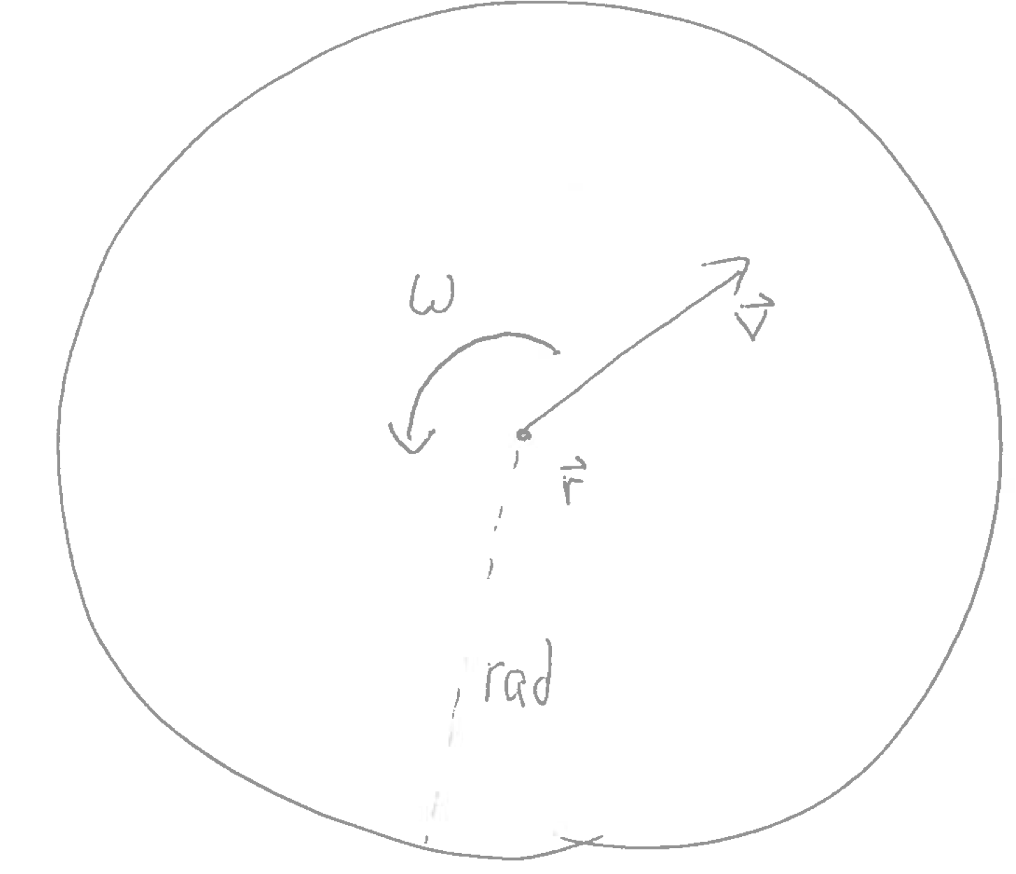
rx, ry, rz, vx, vy, vz, rad, alpha, beta, gamma, omex, omey, omez, info
For each particle, we are given information regarding
info represents an additional variable which can be specified by the user using DPMBase::getInfo. By default, info represents the species index, which stores information regarding the particle’s material/contact properties.The sequence of output lines described above is then repeated for each time step.
It should be noted that the above is the standard output required for three-dimensional data; for two-dimensional data, only five items of information are given in the initial line of each time step:
N, time, xmin, zmin, xmax, zmax
and eight in the subsequent N lines:
x, z, vx, vz, rad, qz, omez, xi
The fstat is predominantly used to calculate stresses.
The .fstat output files follow a similar structure to the .data files; for each time step, three lines are initially output, each preceded by a ‘hash’ symbol (#). These lines are designated as follows:
  # time, fstatVersion
  # xmin ymin zmin xmax ymax zmax
  #
where time is the current time step adn fstatVersion the version number of the output format (currently one, as it has been changed once). The values provided in the second and third line ensure backward compatibility with earlier versions of Mercury, but are not used for analysis.
This initial information is followed by a series of Nc lines corresponding to each of the Nc particle contacts (as opposed to particles) within the system at the current instant in time. Each of these lines is structured as follows:
time, i, j, cx, cy, cz, delta, deltat, fn, ft, nx, ny, nz, tx, ty, tz
i indicates the number used to identify a given particle andj similarly identifies its contact partner.delta represents the overlap between the two particles,deltat the length of the tangential elongation [Reference missing].i is split into a normal and tangential component, \(\vec{f}={\tt fn}\cdot\hat{n}+{\tt fn}\cdot\hat{t}\), where \(\hat{n}=({\tt nx}, {\tt ny}, {\tt nz})\) and \(\hat{t}=({\tt tx}, {\tt ty}, {\tt tz})\) denote unit vectors normal and tangential to the contact plane, respectively.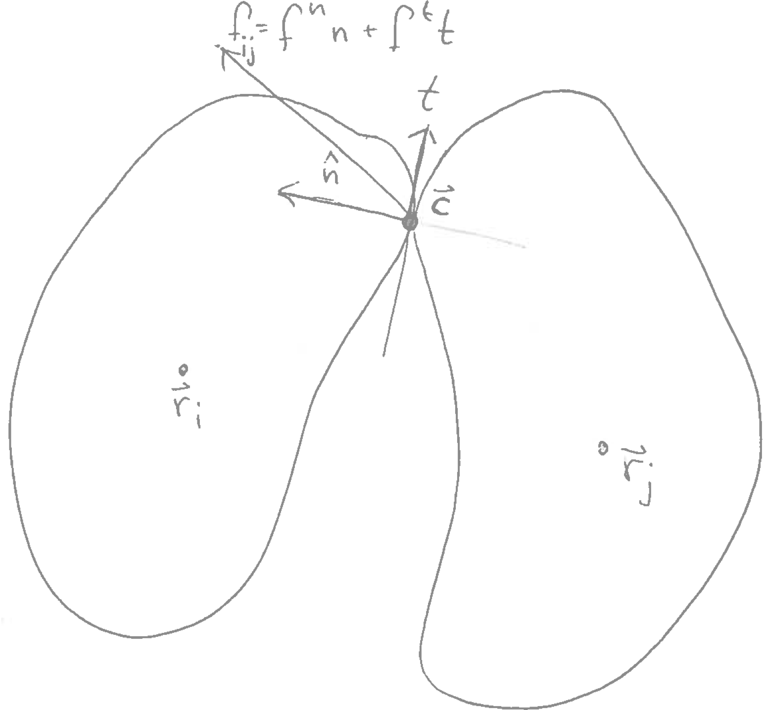
f
We begin by discussing the manner in which Mercury data can simply be ‘visualised’ - i.e. a direct, visual representation of the motion of all particles within the system produced.
ParaView may be downloaded from http://www.paraview.org/download/ and installed by following the relevant instructions for your operating system. On Ubuntu, it can simply be installed by typing
sudo apt-get install paraview
In order to visualise the data using Paraview, the data2pvd tool can be used to convert the ‘.data' files output by Mercury into a '.pvd' Paraview datafile and several VTK (.vtu) files. We will now work through an example, using data2pvd to visualise a simple data set produced using the example code ChuteDemo. From your build directory, go to the ChuteDemos directory:
and run the ChuteDemo code:
Note: if the code does not run, it may be necessary to first build the code by typing:
Once the code has run, you will have a series of files; for now, however, we are only interested in the '.data' files.
Since data2pvd creates numerous files, it is advisable to output these to a different directory. First, we will create a directory called chute_pvd:
We will then tell data2pvd to create the files in the directory:
In the above, the first of the three terms should give the path to the directory in which the data2pvd program is found (for a standard installation of Mercury, the path will be exactly as given above); the second is the name of the data file (in the current directory) which you want to visualise; the third gives the name of the directory into which the new files will be output (‘chute_pvd’) and the name of the files to be created ('chute').
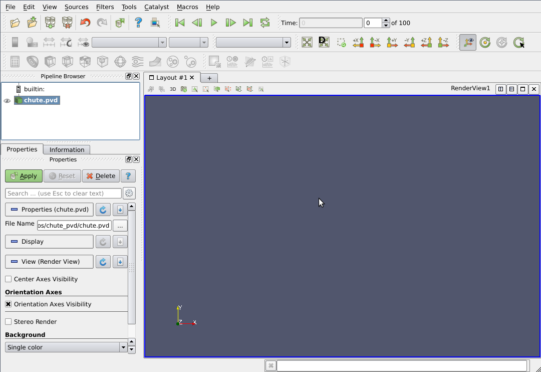
Once the files have been successfully created, we now start ParaView by simply typing:
Which should load a screen similar to the one provided below:
Note: for Mac users, ParaView can be opened by clicking 'Go', selecting 'Applications' and opening the file manually.
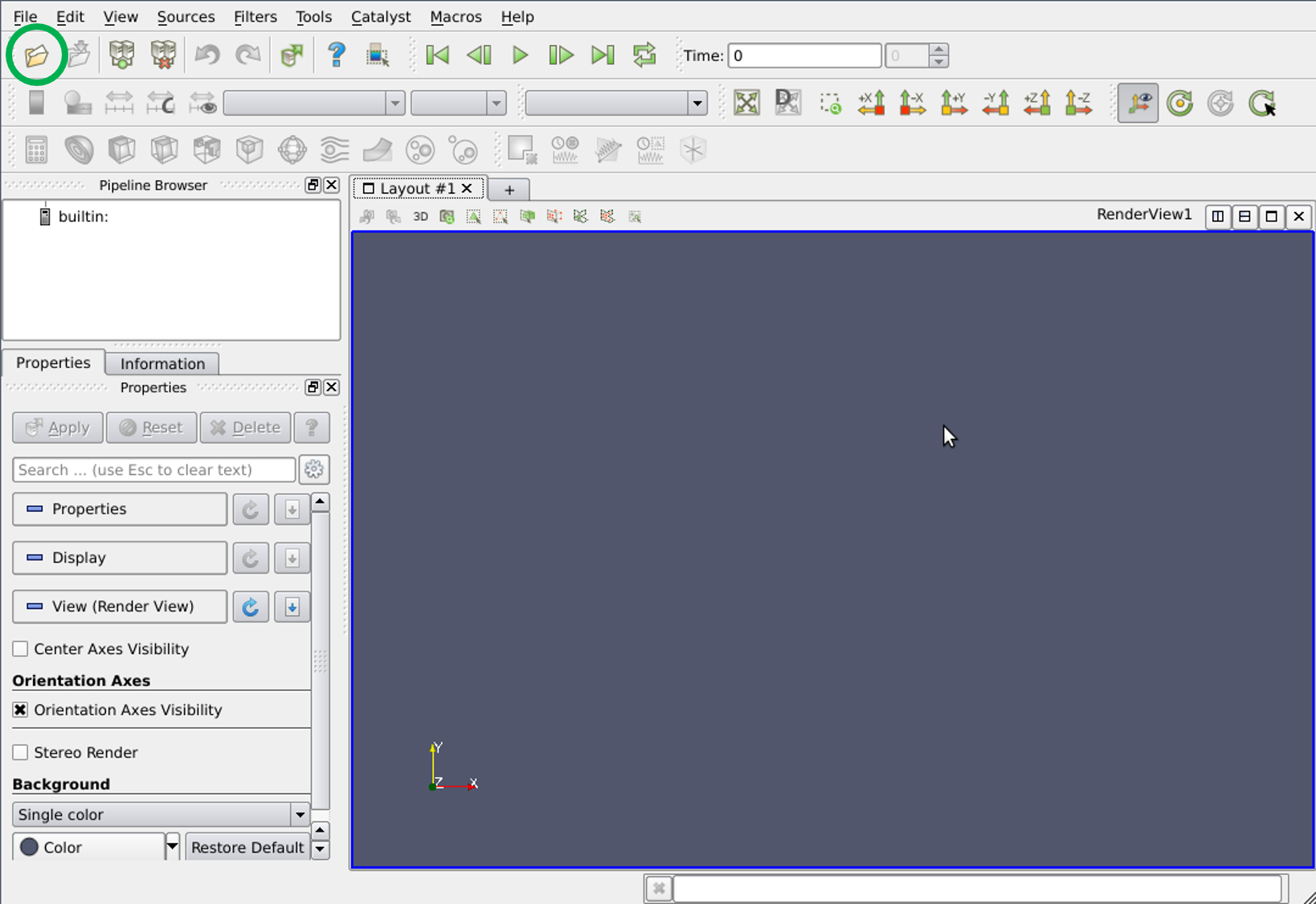
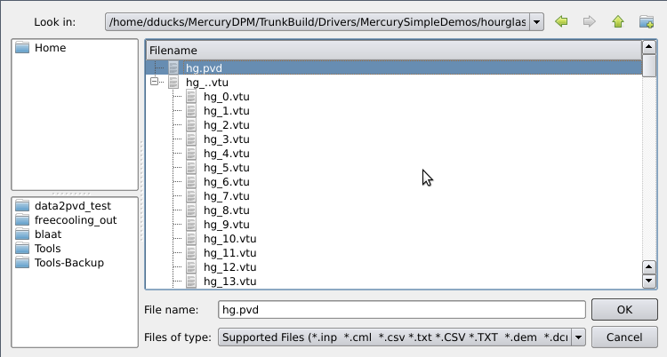
The next step is to open the file by pressing the folder icon circled in the above image and navigating to the relevant directory using the panel shown below.
Here, you can choose to open either the ‘.pvd’ file, which loads the entire simulation, or the '.vtu' file, which allows the selection of a single timestep.
For this tutorial, we will select the full file - ’chute.pvd'.
On the left side of the ParaView window, we can now see chute.pvd, below the builtin in the Pipeline Browser.
Click ‘Apply' to load the file into the pipeline.
Now we want to actually draw our particles. To do so, open the 'filters' menu at the top of the ParaView window (or, for Mac users, at the top of the screen) and then, from the drop-down list, select the 'common' menu and click 'Glyph'.
In the current case, we want to draw all our particles, with the correct size and shape. In the left-hand menu, select 'Sphere' for the ‘Glyph Type’, 'scalar' as the Scale Mode (under the ‘Scaling’ heading) and enter a Scale Factor of 2.0 (Mercury uses radii, while ParaView uses diameters).
Select 'All Points' for the ‘Glyph Mode’ under the ‘Masking’ heading to make sure all of our particles are actually rendered. Finally press 'Apply' once again to apply the changes.
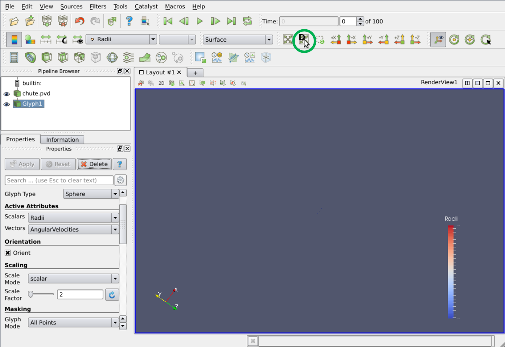
In order to focus on our system of particles, click the 'Zoom to data' button circled in the image above.
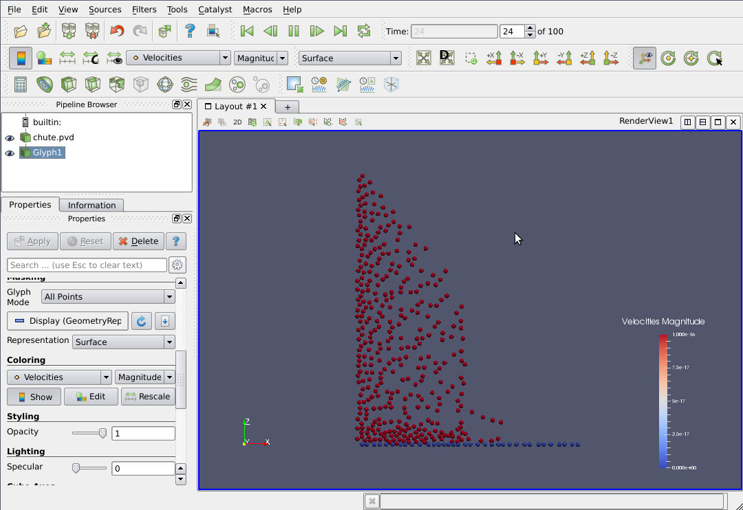
The particles can then be coloured according to various properties; for the current tutorial, we will colour our particles according to their velocities. To do this, with the 'Glyph1' stage selected, scroll down in the properties menu until you find 'Colouring' and select the 'Velocities' option.
The colouring can be rescaled for optimal clarity by pressing the ‘Rescale' button in the left hand menu under the ‘Colouring’ heading.
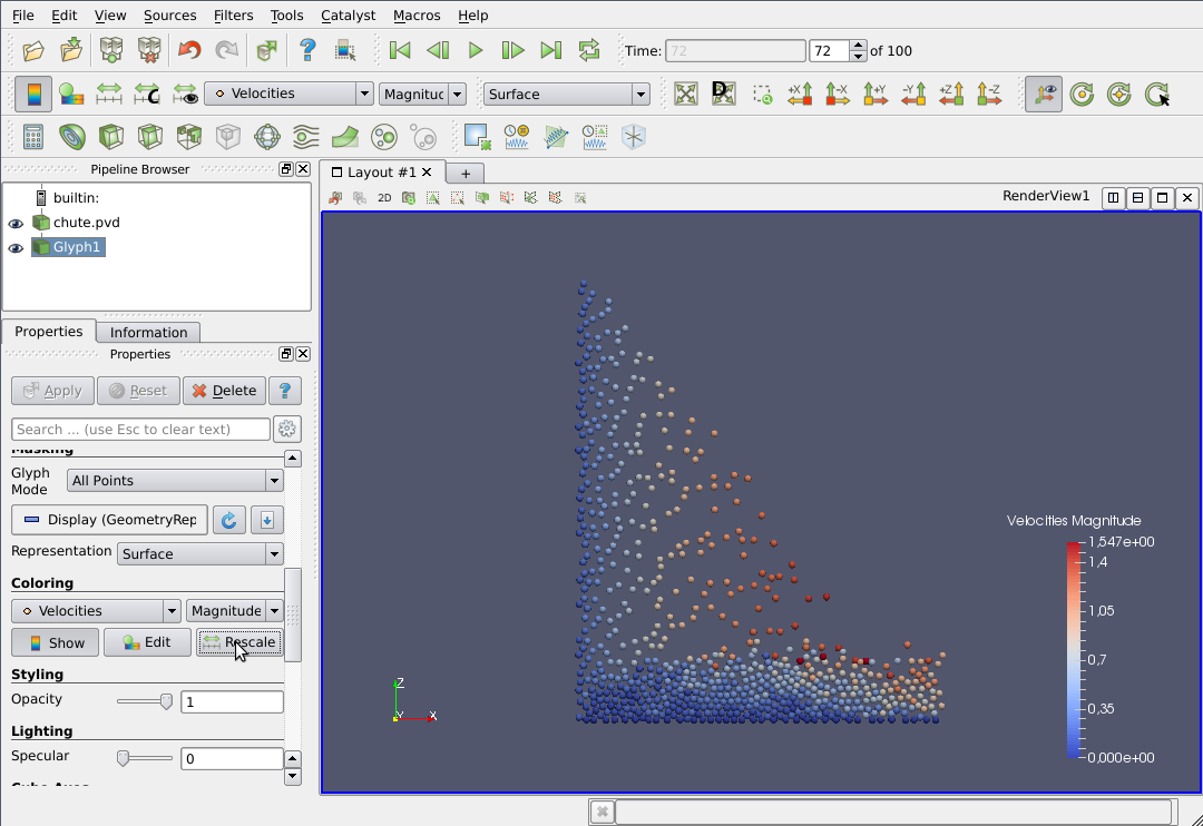
We are now ready to press the 'play' button near the top of the screen and see the system in motion!
The ParaView program has endless possibilities and goes way beyond the scope of this document. Please consult the ParaView documentation for further information.
In the MercuryCG folder (MercuryDPM/MercuryBuild/Drivers/MercuryCG), type ‘make fstatistics’ to compile the ‘fstatistics’ analysis package.
For information on how to operate fstatistics, type ‘./fstatistics -help’.
The Mercury analysis package are due to be upgraded in the upcoming Version 1.1, at which point full online documentation and usage instructions will be uploaded.
If you experience problems in the meantime, please do not hesitate to contact a member of the Mercury team.