|
|
|
|
fstatistics is a postprocessing tool: it takes an existing data set, consisting of a restart and one or more data and fstat files, and applies the coarse-graining formulations to it. The output is stored in a stat file, which can then be read by gnuplot or Matlab (via the loadstatistics.m file in Source/Matlab/thomas/) to be visualised.
This document details how to use fstatistics as a post-processing tool for coarse-graining. It can also be used as a live tool, analysis the data while the simulation is still running, you have to use statistics_while_running.cpp. First, we provide the basic functionality, then show some examples, then the more complex operations are introduced.
To explain the basic syntax of fstatistics, assume that you have the following three files: filename.restart, filename.data and filename.fstat that you want to analyse. To analyse this data,
For simplicity, I assumed here that the data files are in the folder Build/Drivers/MercuryCG/. If the data is in another folder, then you have to use the command ./fstatistics $dir/filename, where $dir is the name of the directory.
By default, fstatistics outputs the time- and space-averaged values of several continuum fields (density, momentum, stress, and a couple more). This output is shown in the command window, as well as stored in the output file named filename.stat.
This is best illustrated by an example: Compile and run the code NewtonsCradleSelfTest, which is in the same directory as fstatistics, and look at its documentation to familiarise yourself with the simulation. Then run ./fstatistics NewtonsCradleSelfTest. The output to the screen shows you the time- and space- averaged values for several continuum fields:
You can see that the volume fraction is 0.523599, the density is 1 mass/length^3, while the momentum nearly vanishes, which agrees with the simulation data.
Note that fstatistics returns the momentum instead of the velocity, as momentum has a primary definition as a coarse-grained variable, while velocity is computed by dividing two existing coarse-grained fields (momentum and density). Generally, fstatistics only outputs the primary coarse-grained variables, and the user is expected to compute any secondary fields afterwards. However, the Matlab script loadstatistics.m provides an extended set of primary and secondary variables
The output file consists of a two-line header followed by several lines of data. For the example above, the output is:
The first line details the different fields that are computed by fstatistics, e.g. volume fraction Nu, bulk density Density and the three momentum components MomentumX MomentumY MomentumZ.
The second line details the coarse-graining parameters, mainly the spatial coarse-graining width w.
The third line shows the time step (or time intervall at which the data is taken); in this case, the data is time averaged from t=0 to t=8.
The remaining lines contains the coordinate of a point and the values of the continuum fields at that point (in the order specified in line 1, so colume 1-3 is the point's coordinate, column 4 is volume fraction, column 5 density, column 6-8 momentum). For globally averaged values, there is only one line of data, with the point's coordinate set to the middle of the domain.
However, fstatistics can do much more than return global averages of the continuum fields. In the following, several commonally used options are discussed.
The output file can be modified by adding additional arguments to the command line. E.g. you can use the -timeaverage command, which takes a boolean (0 or 1) as argument (the default value is 1):
This tells fstatistics to turn off time-averaging. The output file now contains data from several consecutive time steps:
The coarse-graining formulations can return data which is averaged over all spatial coordinate directions (as shown in the previous examples) or only in certain spactial directions. Note, the CG formulation returns fields at ALL points in space; however, we have to evaluate these continuum fields at a final number of 'grid points'. Use the -stattype [O,X,Y,Z,XY,XZ,YZ,XYZ] and -n [double] commands to produce spatially resolved fields:
This produces data that is resolved in the z-coordinate (but averaged in t, x and y). The 'n'-options means a 100 different z-values are evaluated, evenly spread over the domain. The output file now contains 100 lines of data, one for each z-value:
By default, the code uses the radius of the first particle in the restart file as the coarse-graining width, and a cut-off Gaussian coarse-graining kernel. Use the commands -cgtype [Gaussian,Lucy,Heaviside] and -w [double] to change these defaults, e.g.
This produces z-resolved data using a Lucy kernel with a narrow cutoff radius of 0.5 (one particle radius). For an explanation of what a kernel function is, please see the section of the maths of coarse-graining MercuryCG: Post-processing discrete particle data using the coarse-graining formulation (in development)
We can now visualise this data using e.g. gnuplot:
The result is a density field with peaks at the particle centre and vanishing at a distance of 0.5 from the particle centre: 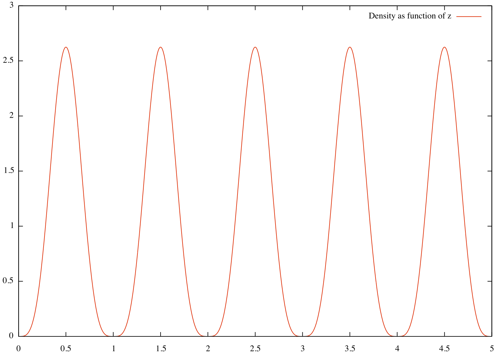 A second example
creates 3D fields (not very sensible for this example) evaluation on a grid which is 10 by 2 by 2. When generating multi-dimensional data -n uses a uniform grid.
By default, fstatistics uses evaluates all time steps. However, often time-averaging over a particular time interval is desired, e.g. to look at steady-state data only, or to reduce the computational effort. You can use the -tmin [double] and -tmax [double] commands to set a time interval on which the coarse graining should be applied:
Similarly, one can change the spatial mesh on which the coarse-graining is evaluated: By default, fstatistics assumes that you want to evaluate the continuum fields on the domain size defined in the restart file. To change this, use the commands -x [double] [double], -y [double] [double] and -z [double] [double]:
-w_over_rmax [double]: Set the averaging width in multiples of the radius of the largest particle in the restart file.
-nx [integer], -ny [integer], -nz [integer]: Specifies the amount of grid points in a specific coordinate direction; use -n [integer] to set all 3 directions at once.
-h [double], -hx [double], -hy [double], -hz [double]: Alternatively to setting the amount of grid points with -n, one can also specify the mesh size instead. E.g. for a domain of width 3, -h 0.01 is equivalent to setting -n 300. Use -h to set the mesh size of all 3 directions at once, -hx, -hy or -hz to specify the mesh size in a specific coordinate direction.
-indSpecies [integer]: Evaluates only data pertaining to a particular Species. Useful for the coarse-graining of mixtures.
-rmin [double], -rmax [Mdouble]: Evaluates only data pertaining to particles above or below the specified radius, respectively.
-hmax [double]: Evaluates only data pertaining to particles below the specified height.
-walls [uint]: only takes into account the first n walls
-verbosity [0,1,2]: amount of screen output (0 minimal, 1 normal, 2 maximal)
-verbose: identical to -verbosity 2
-stepsize [integer]: Evaluates only ever n-th time step. Useful to reduce the amount of computational effort.
-o [string]: Changes the name of the output file to string.stat
-timevariance [bool]: Prints the time variance; only for time averaged data.
-gradient: Prints the first derivative of each statistical value