MercuryCG: Post-processing discrete particle data using the coarse-graining formulation (in development)

This feature is still in development, so the documentation is meant for developers only. However, anyone is welcome to give it a try.

MercuryCG is a new implementation of the coarse graining toolbox fstatistics, and will replace this toolbox in the near future.

MercuryCG is a postprocessing tool: it takes an existing data set, consisting of a restart and one or more data and fstat files, and applies the coarse-graining formulation to it. The output is stored in a stat file, which can then be read by gnuplot or Matlab (via the readMercuryCG.m file in Drivers/MercuryCG/) to be visualised.

This document details how to use MercuryCG as a post-processing tool. Note, coarse graining can also be applied during a MercuryDPM simulation, analysing the data while the simulation is still running; to do this, see the CGHandler documentation.

Basic syntax

First, we provide the basic syntax, then show some examples. Finally, more complex operations are introduced.

Assume you want to analyse the output files of the Driver's code NewtonsCradleSelfTest, located in the folder Drivers/MercuryCG. To create the file, run the simulation using make SquarePackingSelfTest && ./SquarePackingSelfTest in said folder). The simulation produces two output files that MercuryCG needs: SquarePackingSelfTest.data and SquarePackingSelfTest.fstat. To analyse this data,

  • change to the folder Drivers/MercuryCG/ in the build directory,
  • compile MercuryCG
    make MercuryCG
  • run the following command
    ./MercuryCG SquarePackingSelfTest

Note: If the data is in another folder than Drivers/MercuryCG/, you have to prepend the file path to the file name. For example, to analyse the output files of LeesEdwardsSelfTest in the folder MercurySimple demos, use the command

./MercuryCG ../MercurySimpleDemos/LeesEdwardsSelfTest
[Lees:headers]
Definition: LeesEdwardsSelfTest.cpp:34

With the above arguments, MercuryCG outputs spatially-averaged continuum fields for each time step in the data/fstat files into a file named 'SquarePackingSelfTest.stat`. For a quick check of the output, the spatially-averaged results from the last written timestep are outputted to the screen

Spatial averages: VolumeFraction 0.785398 Density 1 Momentum 0 -5.6968e-07 0 ...

Note that MercuryCG returns the momentum instead of the velocity, as momentum has a primary definition as a coarse-grained variable ( \(\vec{j}=\sum_i m_i\vec{v}_i\phi_i\)), while velocity is computed by dividing two "primary" coarse-grained fields (momentum and density, \(\vec{V}=\vec{j}/\rho\)). Generally, MercuryCG only outputs primary coarse-grained variables, as they are well-defined even if no particles are present. The primary fields are also the most relevant for any macroscopic theory based on conservation principles, as they have well-defined averaging properties (they can be thought of as the density of a microscopic quantity). Secondary fields like velocity can be constructed by combining the primary fields. The script readMercuryCG.m reads the primary variables into Matlab and constructs several secondary variables (velocity, kinetic stress, temperature, etc).

Output format

The output file consists of a two-line header followed by several lines of data. For the example above, the output is:

CG<O> n 1 1 1 min 0 0 -0.5 max 5 5 0.5 width 1 Lucy cutoff 1
time 2:VolumeFraction 3:Density 4-6:Momentum ...
0 0.785398 1 0 0 ...
0.4 0.785398 1 0 6.72166e-05 ...
0.6 0.785398 1 0 -1.53499e-05 ...
0.8 0.785398 1 0 3.09892e-06 ...
1 0.785398 1 0 -5.83261e-07 ...
const unsigned n
Definition: CG3DPackingUnitTest.cpp:32
Evaluates time-resolved continuum fields and writes the data into a stat file.
Definition: CG.h:76

The first line outputs a few properties you need to interpret the remaining file output:

  • CG: the standard CG class was used, which evaluates each time step separately (see also TimeAveragedCG and TimeSmoothedCG)
  • '<O>': the coordinate type O was used, which returns spatial averages (see also X, XY, XYZ, etc) The first line details the different fields that are computed by fstatistics, e.g. volume fraction Nu, bulk density Density and the three momentum components MomentumX MomentumY MomentumZ.
  • min 0 0 -0.5 max 5 5 0.5: the spatial domain
  • n 1 1 1: a 1x1x1 mesh of values was used, which is the only option for spatially averaged statistics.
  • width 1: the coarse-graining width
  • Lucy: the type of coarse-graining function (see Gaussian, Lucy, Linear and Heaviside)
  • cutoff 1: the coarse-graining width

The second line specifies the time/space coordinates and fields computed by MercuryCG and the respective columns.

The remaining lines contains the coordinates and the values of the continuum fields at these coordinates.

Advanced options

MercuryCG can do much more than return global averages of the continuum fields. In particular, it can extract local continuum fields at specific spatial coordinates. The behavior of MercuryCG is controlled via command line arguments; the most commonly used options are discussed in more detail below.

Temporal averaging

The output file can be modified by adding additional arguments to the command line. E.g. you can use the -timeaverage command:

./MercuryCG SquarePacking -timeaverage
Definition: SquarePackingSelfTest.cpp:35

This tells MercuryCG to time-average. The output file now looks like this:

TimeAveragedCG<O> min 0 0 -0.5 max 5 5 0.5 n 1 1 1 width 1 Lucy cutoff 1
time 2:VolumeFraction 3:Density 4-6:Momentum ...
1 0.785398 1 0 -2.3681e-05 ...
Evaluates time-averaged continuum fields and writes the data into a stat file.
Definition: TimeAveragedCG.h:59

Spatially-resolved fields

The coarse-graining formulations can extract local continuum fields, whose value depends on the spatial coordinate. You can extract spatially resolved fields using the arguments -coordinates XYZ -n 2 -timeaverage. This creates a 2x2x2 grid of values over the domain and evaluates the continuum fields at each of those points. Note, the grid is not part of the cg formulation itself: CG returns field values at all points in space; but numerically we can only evaluate the continuum fields at a final number of points. The output file now contains 8 lines of data, one for each z-value:

TimeAveragedCG<XYZ> min 0 0 -0.5 max 5 5 0.5 n 2 2 2 width 1 Lucy cutoff 1
time x y z 5:VolumeFraction 6:Density 7-9:Momentum ...
1 1.25 1.25 -0.25 0.744721 0.948208 0 -1.71359e-05 ...
1 1.25 1.25 0.25 0.744721 0.948208 0 -1.71359e-05 ...
1 1.25 3.75 -0.25 0.744362 0.947751 0 -2.94495e-05 ...
1 1.25 3.75 0.25 0.744362 0.947751 0 -2.94495e-05 ...
1 3.75 1.25 -0.25 0.744721 0.948208 0 -1.71359e-05 ...
1 3.75 1.25 0.25 0.744721 0.948208 0 -1.71359e-05 ...
1 3.75 3.75 -0.25 0.744362 0.947751 0 -2.94495e-0 ...
1 3.75 3.75 0.25 0.744362 0.947751 0 -2.94495e-05 ...
...

You can also choose to spatially resolve only specific spatial coordinates and average over the remaining ones. Use the arguments '-coordinates [O,X,Y,Z,XY,XZ,YZ,XYZ]' to modify this behaviour.

By default, the code uses the coarse-graining width 1, and a Lucy coarse-graining function. Use the arguments -function [Gaussian,Lucy,Linear,Heaviside] and -w [double] to change these defaults. For an explanation of what a kernel function is, please see the section on the maths of coarse-graining.

Visualisation

The following command produces z-resolved data using a Lucy kernel with a narrow cutoff radius of 0.5 (one particle radius).

./MercuryCG SquarePacking -coordinates Z -n 100 -function Lucy -w 0.5
@ Z
Definition: StatisticsVector.h:42

We can now visualise this data using e.g. gnuplot:

gnuplot> p 'SquarePackingSelfTest.stat' u 2:4 w l
void gnuplot(std::string command)
Plots to a gnuplot window.
Definition: MiscHelpers.cc:38

The result is a density field with peaks at the particle centre and vanishing at a distance of 0.5 from the particle centre: 
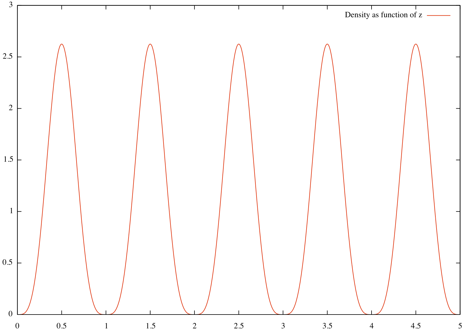
Alternatively, you can visualise the data in Matlab:

$ data = readMercuryCG('SquarePackingSelfTest.stat')
$ plot(data.z,data.Density)

Command line manual

You can obtain a full list of command line options by typing the -help command:

./MercuryCG -help
DESCRIPTION
MercuryCG is the postprocessing tool for extracting coarse-grained fields from particle data.
SYNTAX
You need to specify the base name of the MercuryDPM output files (data/fstat or restart files) that should be analysed.
Additional arguments can be specified as [-option value] pairs:
./MercuryCG name [-option value]
EXAMPLES OF USE
1) To extract spatially-averaged continuum fields (i.e. the fields are functions of t only) from
the output files name.*, use the following command:
./MercuryCG name -coordinates O
2) To extract fully-resolved continuum fields (i.e. the fields are functions of x, y, z and t) from the output files name.* on a 10x10x10 spatial grid, use the following command
./MercuryCG name -coordinates XYZ -n 10
OPTIONS
-help
Outputs a usage message and exits
-coordinate value, -stattype value
Determines which spatial dimensions should be resolved.
Possible values are O, X, Y, Z, XY, XZ, YZ, XYZ, default is O.
-function value, -cgtype value
Determines the cg function.
Possible values are Gauss, Heaviside, Linear, Lucy, default is Lucy.
-fields value
Determines which fields should be extracted.
Possible values are StandardFields, LiquidMigrationFields, GradVelocityFields, default is StandardFields.
-timeaverage
If this option is specified, the data will be time-averaged.
-timesmooth
If this option is specified, the data will be coarse-grained in time.
-n value
Creates a spatial grid of n elements in each resolved dimension.
Equivalent to '-nx value -ny value -nz value'.
-nx value, -ny value, -nz value
Specifies the amount of elements in each spatial direction.
Will be ignored if the spatial direction is not resolved.
Coarse-grained fields will be evaluated at the midpoints of each element.
By default, the domain is equal to the spatial domain of the DPM, as specified in the restart file (or data file if no restart file is given). However, the domain of the grid can be specified by the -x, -y, -z options.
For example, for '-x 0 10 -nx 5', the cg fields will be evaluated at x=1,3,5,7,9.
-h value
Allows you to specify the element size in stead of the number of elements of the spatial grid.
Equivalent to '-hx value -hy value -hz value'.
-hx value, -hz value, -hz value
Allows you to specify the element size in stead of the number of elements of the spatial grid.
Equivalent to -nx ceil((maxX-minX)/value), where [minX,maxX] is the domain of the spatial grid.
-n value
Creates a spatial grid of n elements in each resolved dimension.
Equivalent to '-nx value -ny value -nz value'.
-x value1 value2, -y value1 value2, -z value1 value2
Specifies the domain of the spatial grid on which the coarse-grained fields will be evaluated.
For example, for '-x 0 10 -nx 5', the cg fields will be evaluated at x=1,3,5,7,9.
-t value1 value2, -tmin value, -tmax value
Specifies the minimum and maximum time values on which the cg fields will be evaluated.
-o value
Specifies the name of the output file in which the cg fields are written.
By default, the output file will be named 'name.stat'.
@ XY
Definition: StatisticsVector.h:42
@ XZ
Definition: StatisticsVector.h:42
@ YZ
Definition: StatisticsVector.h:42
@ Y
Definition: StatisticsVector.h:42
@ X
Definition: StatisticsVector.h:42
@ XYZ
Definition: StatisticsVector.h:42
@ O
Definition: StatisticsVector.h:42
In this file a cubic packing of 5^3 particles in a tri-axial box is created and allowed to settle und...
Definition: HGridUpdateUnitTest.cpp:30
Definition: restart2.cpp:29
const std::complex< Mdouble > i
Definition: ExtendedMath.h:51
std::string name
Definition: MercuryProb.h:48

Full-scale Images